
I feel that today’s network lags are not normal… But is it really so? Or is it my mind playing tricks on me? The KS test (Kolmogorov-Smirnov) is a practical tool to provide objective answers to such questions. Here is a practical intro for Python programmers with little background in statistics.
Another example: let’s examine several groups of events that happened in some IT system. Is there a significant difference between them? Answering questions like this has broad impact:
- infrastructure management: comparing groups of incidents can tell the system health, indicate anomalous periods and improve long-term business parameters of a project (SLA)
- ITSM / ITOM / AIOps: comparing logfile records from various periods allows to measure frequency, stability and repeatability of technical events, and generate alerts in the anticipation of problems
- application management: comparing incidents from various groups of users (reporters, pilots) tells how quickly the employees grow in maturity, when they need training, and what degree of trust can be given to their judgment
This last bulletpoint is a follow-up to the previous article ‘are people fair’. We will work on the example from that article, where we discussed the chart below. It represents distribution of a certain behavior of three groups of users: how they rank incident priorities. Are these groups significantly different in behavior, or not?
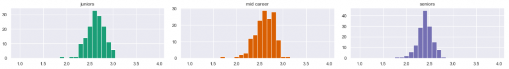
A number of statistical methods can help. Our data is numeric (not categorical), continuous, and not normal (the distribution does not resemble the Gaussian bell curve). Therefore we cannot use normality tests, or chi-square test for goodness of fit. We could use the Kolmogorov-Smirnov test, also known as KS test, as well as Shapiro-Wilk test and Anderson-Darling test. In this article will focus on the the KS test only.
What is KS test good for
KS test is a powerful tool that exists in two versions. The 1-sample KS test can tell us whenter the sample is drawn from a certain distribution. This can tell us, for instance whether today’s incidents are anomalous compared to the annual average.
The 2-sample KS test can tell us whether 2 independent samples are drawn from the same continuous distribution. In the practical terms of our example, this can tell whether two groups of users behave differently.
Because the theoretical foundations of the KS test have been nicely covered elsewhere (thank you, Charles Zaiontz), here I will skip that and simply proceed to a very practical introduction for using it in Python.
Quick start: using the KS test in Python
Usage of scipy.stats.kstest() is quite easy, but the interpretation is not. Before using it for real decision making, it is a good idea to play with the tool to get some feeling. I recommend to put our example aside (we will come back to it later) and run the following simple experiments with abstract data. First, let’s draw a random sample from a normal distribution, and apply the 1-sample KS test to it, comparing it to… normal distribution again. Of course we expect the KS test to say ‘yes, it looks like that sample does come from this distribution‘. Here is the code (and no more code in this article, promise):
import scipy.stats, random, numpy as np
x = np.random.normal(loc=0.0, scale=1.0, size=10000)
s = np.array(random.sample(x.tolist(), 100))
kstest(rvs = s, cdf = 'norm')
And the output is:
KstestResult(statistic=0.027649445938028427, pvalue=0.8392203783748184)The KS test responded with two numbers: KS statistics, and the p-value. That looks… cryptic. Why it cannot provide a simple yes/no answer? Why we received two answers instead of one? Which number to take into account: statistics, p-value, or any, or both? I am proceeding straight to the answers.
Most importantly: for practical purposes, you can use any of those numbers to interpret the answer. Looking at just one of them is enough. So, either learn to interpret the KS statistics, or learn to undersand the p-value. The 1-sample KS statistics can be interpreted using this table , followed by some simple mathematical operations. For beginners, using p-value is easier, because it can be interpreted immediately with no tables and no maths. The meaning: the p-value provides probability of a ‘yes’ answer (where ‘yes‘ means that the sample matches the distribution, and ‘no’ means no match). So, our p-value above says that there is 84% chance that our sample came from normal distribution. (this is not fully correct, but it works as practical simplification of the proper definition of p-value). This also explains why the KS test cannot give us a yes/no answer. Instead, it provides the level of certainty of a yes.
So, we have seen that the KS test works. It said it was 84% sure that the sample matched the distribution. Fair enough. But how about running this again? We may end up scratching our heads over this result:
KstestResult(statistic=0.052007044779638356, pvalue=0.12916012924670686)
Now the KS test said it was only 12% sure. What happened, is it broken?
Why it fails
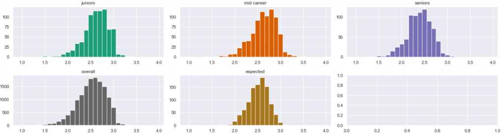
It is not broken. It just so happens, that our random sample is, by definition, random. So the second time we have generated a second, different sample. And it might be that the KS test was less confident. If so, then to what extent can we trust this tool? To get a feeling, let’s draw a random sample 1000 times, and see the distribution of the result set. Below in Figure 2 is my result.
In the middle diagram are the p-values. Large is good. How large is large enough? Here a small surprise for those who do not work with statistics: in practice, we often assume that the values above 0.05 (the red vertical line) are yeses, and the values below mean no. We then speak of alpha 5%, or confidence level of 95%. If this surprises you ( why it’s 95/5 rather than 50/50?), read more about statistical hypothesis testing.
In the leftmost diagram is the KS statistics. Small is good. Values below the red line (the critical value) can be interpreted as yeses. I will not discuss the KS statistics in this article, so you have to believe me. In the rightmost chart we can see how those two sets (KS statistics and p-value) correspond to each other.

The observations are: as expected, 95% of the samples received p-value above 0.05, so were ranked as yeses. The rightmost chart can also tell us something important: samples ranked negatively with p-value, were also ranked negatively with KS statistics. So it does not matter which one of the two we analyze (I am simplifying again, but in practice it is so). Hence, we will skip the KS statistics from now on, as it is more complicated, and focus on the p-value.
So, why and how often does it fail? The answer is: it is up to us. If we assume confidence level of 95%, the test will result in a False Negative in 5% of the cases. We can reduce this to 1% or even 0.1%, but doing so will increase the rate of False Positives.
Forcing the KS test to fail
Now what happens if we try to cheat the KS test?
To illustrate what I want to simulate now: assume the normal distribution represents a group of healthy people with averge body temperature is 36.6 degree Celcius, noting that individual deviations are possible. Now suppose we measure one new individual, and his temperature is higher by 0.15, that is 36.75 degrees. Can we tell that he is sick? Probably not, because this is a very small difference. But if we had more such measurements? Suppose we received a sample of 100 people from a group where the average temperature was 36.75 (with individual deviations). Will the KS test tell the difference, correctly stating that this group is statistically different (probably sick)? Let’s see.
To simulate this, I will now draw a sample of 100 measurements from a different distribution, with the mean 0.15 rather than 0 (in the Python code below, note the loc parameter) . But the KS test still expects the mean 0. Will it tell the difference?
import scipy.stats, random, numpy as np
x = np.random.normal(loc=0.15, scale=1.0, size=100)
s = np.array(random.sample(x.tolist(), 100))
kstest(rvs = s, cdf = 'norm')
As we already learned, one result will not tell us anything. But let’s repeat this 1000 times and see the resulting p-values distribution:

Interesting. The KS test still thinks that most of the samples are fine. However, it is now confident in about 75% of the cases. 25% cases fall below the alpha of 0.05: 25%. There, the KS test realized something was wrong. Now, how about if we increase the sample size to 1000? Here:

Now the certainty has improved radically. In 98.6% of the cases the KS test resulted in p-value below 0.05, which we interpret as a ‘no’. In other words: one measurement of 36.75 does not make a difference, 100 measurements cause some concern, and 1000 such measurements causes certainty thatthe situation is not normal. The important conclusion: The larger the sample, the higher the certainty. With big samples, even tiny deviations from the original population will be detected.
Comparing 2 samples
So far, we worked with 1-sample KS test, comparing the sample to the normal distribution. But our original task is different: we should compare two samples. For this we shall use the 2-sample KS test. It behaves similarly. Just to be sure, let’s repeat the experiment. We will now run the KS test to compare two samples, both from normal distribution, to each other.
from scipy.stats import ks_2samp
s1 = np.random.normal(loc = loc1, scale = 1.0, size = size)
s2 = np.random.normal(loc = loc2, scale = 1.0, size = size)
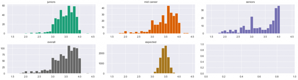
(ks_stat, p_value) = ks_2samp(data1 = s1, data2 = s2)We have run this 1000 times, assuming alpha 0.05, and here is the aggregated result of p-values and KS-statistics:

The chart looks a bit different but it does not matter. As expected, the test interprets 95% results as yeses. If we want 99% hit, we should set alpha as 0.01.
Having gone through these experiments, we should have some confidence in using 2-sample KS test as productive tool. The key takeaways are:
- it is safe to only interpret the p-value and ignore the KS-statistics
- the p-value is like probability that the two populations are the same. Above 5% means the samples are indistinguishable, and anything below means that they are different (the proper wording here is: if the result falls within the confidence interval of 95%, then we cannot justify rejecting the null hypothesis H0 stating that there is no significant difference between the samples)
- larger sample size increases the certainty of the KS test
Synthesis: back to the original example
Now equipped with knowledge, we can go back to the samples from our previous article. There, we compared three groups of users (juniors, mid-career, and seniors) from two projects: project A and project B. Those people ranked incidents, and we wanted to see if their ranking was fair. We reached tentative conclusion that in the project A, the behavior of all three groups was the same (they were all fair and consistent in judgment), but in the project B, that behavior was different. But those conclusions were based on visual analysis only. Let’s now confirm these findings with statistics, applying the KS test to those samples.
First, project A:
We compared the population of juniors to mid-career, and then to seniors. The KS test results are:

This means that the juniors behave same way as mid-career (p-value 0.999). The difference between juniors and seniors is somewhat bigger, but not big enough to raise concern (p-vaue of 0.14 is still higher than 0.05). Conclusion: all three groups indeed behave the same way, but… I will show something later. And now, Project B:
Again, we compared the population of juniors to mid-career, and then to seniors:

In both cases, the difference is striking. The KS test is quite certain that those populations are different from each other. This confirms the tentative conclusions from the previous article… you think?
However, not quite. Let’s go back to project A, and now compare the expected distribution (brown) to the observed ones. The p-values are:

Note the scientific notation. The p-values are all very low, almost zero. In juniors, it is 0.00025. The interpretation: the observed distributions do not match the expected. How come all observed populations are similar to each other, but in the same time all are different from the expected one?
Business interpretation: in the project A, all three user groups behave the same way. In the same time, we observe with some surprise something we did not spot in the initial visual analysis: all three groups are equally unfair in their ranking of incidents. They have too many extreme rankers, as compared to the expected distribution. However, this is probably not caused by the human factor, because the groups are similar to each other. This can be caused by methodic, business or technical constraints, affecting employees in all groups in the same way.
Summary and Credits
To summarize, the KS test can provide quite a bit of business insight, once you learn how to handle it. It can tell us whether groups of data points (representing events, incidents, users, or records) are different. Good luck!
Credits for this work, again, go to Sopra Steria which provided data for this research. This work is part of our constantly growing expertise in the AIOps domain (that’s Data Science applied to IT Service Management). For any Service Desk, Infrastructure Management, or Application Management project, consider Sopra Steria as your service provider. The Lagoon Data Lake which we internally operate provides an opportunity for comparative analyses. The resulting insight is aimed to optimize your project for performance and cost.